The Lagrange Method for Optimization

The Lagrange method can be used to help us perform optimization by determining the relative weightage of each asset in order to minimize portfolio variance or maximize returns.

First, we need to form a Lagrangian function L(x, λ) augmented by the addition of the constraint functions. Each constraint function is multiplied by a variable, called a Lagrange multiplier.

Let’s consider two cases:

Case 1: Risk Minimization With N Risky Assets

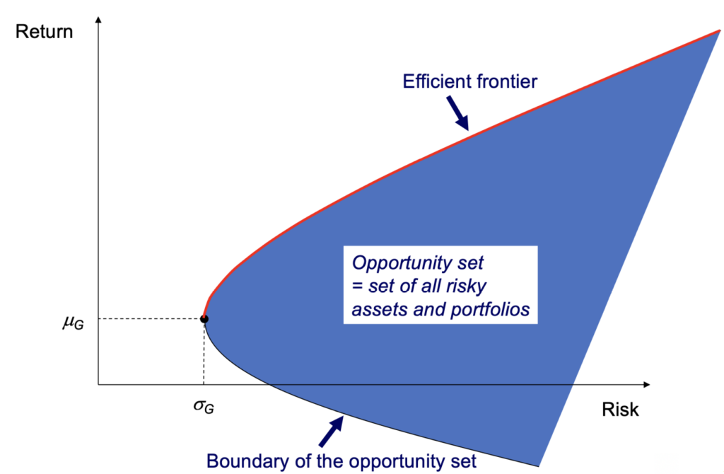
Suppose we want to minimize the variance (i.e. risk) of a portfolio that consists of N risky assets, subject to a minimum level of portfolio return (denoted as m). The opportunity set and efficient frontier is shown below:

We can formulate the problem as

min_\mathrm w \frac{1}{2} \mathrm w'\Sigma \mathrm w

subject to:

\begin{aligned}
\mathrm w'\mu &= m\\\\
\mathrm w'\bold1 &= 1
\end{aligned}

where Σ = covariance matrix, w = vector of asset weights, μ = vector of asset returns, 1 = one vector and m = pre-specified return level.

All vectors are column vectors, while their transposes are row vectors.

The first constraint w’μ = m specifies that the portfolio return must be equal to m, while the second constraint w’1 = 1 specifies that all assets must be invested (i.e. all the weights must sum to 1).

To solve this optimization problem, we form the following Lagrange function and use partial differentiation to solve for the weights vector w:

\begin{aligned}
L(\mathrm w, \lambda, \gamma) &= \frac{}{}\mathrm w' \Sigma \mathrm w + \lambda (m - \mathrm w'\mu)+\gamma(1 - \mathrm w'\bold 1)\\\\
\frac{\partial L}{\partial \mathrm w}(\mathrm w, \lambda, \gamma) &= \Sigma \mathrm w - \lambda \mu - \gamma \bold 1 = 0\\
\mathrm w* &= \Sigma^{-1}(\lambda\mu+\gamma\bold 1)\\\\
\frac{\partial ^2 L}{\partial \mathrm w^2} &= \Sigma > 0\\\\
\end{aligned}

Substituting w* into the two constraints, we get

\begin{aligned}
\mathrm w'\mu &= m\\
\mu'\mathrm w &= m\\
\mu'\Sigma^{-1}(\lambda\mu+\gamma\bold 1) &= m\\
\lambda \mu'\Sigma^{-1}\mu + \gamma \mu'\Sigma^{-1}\bold 1 &= m\\\\
\mathrm w'\bold1 &= 1\\
\bold1'\mathrm w &= 1\\
\bold1'\Sigma^{-1}(\lambda\mu+\gamma\bold 1) &= 1\\
\lambda \bold 1' \Sigma^{-1} \mu + \gamma \bold 1'\Sigma^{-1}\bold 1 &= 1\\\\
\text{Let }A = \bold 1'\Sigma^{-1}\bold 1&\\
B = \mu' \Sigma^{-1} \bold 1 &= \bold 1'\Sigma^{-1}\mu\\
C = \mu' \Sigma^{-1}\mu&\\\\
C\lambda + B\gamma = m&\\
B\lambda + A\gamma = 1&\\\\
\lambda = \frac{Am - B}{AC - B^2}&\\
\gamma = \frac{C - Bm}{AC - B^2}&
\end{aligned}

Case 2: Risk Minimization With N Risky Assets and a Risk Free Asset

The opportunity set and efficient frontier is shown below:

The optimization problem becomes:

min_\mathrm w \frac{1}{2} \mathrm w'\Sigma \mathrm w

subject to:

\begin{aligned}
r + \mathrm w'(\mu - r\bold 1)&= m\\
\end{aligned}

The budget constraint no longer exists as the residual of the wealth not invested in risky assets is now in the risk-free asset. The Lagrange function becomes:

L(\mathrm w, \lambda) = \frac{1}{2} \mathrm w' \Sigma \mathrm w + \lambda(m - r - \mathrm w'(\mu - r\bold 1)) 

After optimization, we get:

\begin{aligned}
\mathrm w* = \frac{(m-r)\Sigma^{-1}(\mu - r\bold 1)}{(\mu - r\bold 1 )'\Sigma^{-1}(\mu - r\bold 1 )  }
\end{aligned}