Note that this post does not summarize everything that’s covered in the book. I am only summarizing what is relevant/new for me.

Table of Contents

Chapter 1: The Whats, Whos, and Whys of Quantitative Trading

Daily work (for a semi-automated operation)

Before the market opened (takes about 2 hours):
- run various programs to download and process the latest historical data
- read company news that came up on the alert screen
- run programs to generate the orders for the day
- launch a few baskets of orders before the market opened
- start a program that will launch orders automatically throughout the day
- update spreadsheet to record the previous day’s profit and loss

Near the market close (about half hour):
- direct the programs to exit various positions
- manually check that those exit orders were correctly transmitted
- close down various automated programs properly

Daily work (for a fully-automated operation)

Monitor and intervene when software and connectivity broke down

Chapter 2: Fishing for Ideas

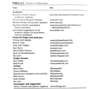
Where Can We Find Good Strategies?

Regarding Trading Capital:
- Minimum initial investment: $50000
- Dividing line between a high- versus low-capital account is $100,000
- Trading futures, currencies, and options can offer you higher leverage than stocks
- Intraday positions allow a leverage of 4, while overnight positions allow only a leverage of 2
- A dollar-neutral portfolio requires twice the capital of a long- or short-only portfolio
- Certain brokers (such as Interactive Brokers) offer a portfolio margin which depends on the estimated risk of your portfolio

I started my life as an independent quantitative trader with $100,000 at a retail brokerage account (I chose Interactive Brokers), and I traded only directional, intraday stock strategies at first… I downloaded only the split-and-dividend-adjusted Yahoo! Finance data…
Quantitative Trading, EP Chan

Sharpe Ratio
- As a rule of thumb, any strategy that has a Share ratio of less than 1 is not suitable as a stand-alone strategy. For a strategy that achieves profitability almost every month, its (annualized) Sharpe ratio is typically greater than 2. For a strategy that is profitable almost every day, its Sharpe ratio is usually greater than 3.

Chapter 3: Backtesting

Backtesting software
- Excel
- Mathlab
- Python
- R
- QuantConnect
  - a web based algo trading platform providing research, backtesting and live trading tools to support strategy creation in C# or Python.
  - Also provides 400TB of financial and alternative data.
  - The open source engine (LEAN) takes into account trade fills, slippage, margin, transaction costs, and bid ask spread to provide realistic backtest results.
- Blueshift
  - integrated platform for research, backtest, and trading offered by QuantInsti.
  - Includes minute level data efree of cost across markets.
  - You can develop your investment or trading strategy in either a Python programming environment or a visual (non programming interface) BUILDER.
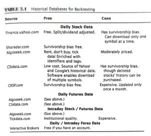
Historical databases for backtesting

Adjusting for dividends
- All prices before the dividends ex-date has to be multiplied by

\frac{C_{T-1}-d}{C_{T-1}}

where d is the dividend per share.

Performance Measurement

Sharpe Ratio
- You need to subtract the risk free rate from your strategy returns in calculating the Sharpe ratio only if your strategy incurs financing costs
  - you do not need to subtract the risk free rate from the returns of a dollar neutral portfolio (as he portfolio is self financing, meaning that the cash you get from selling short pays for the purchase of the long securities. In addition, the margin balance you need to maintain earns a credit interest close to the risk free rate)
  - you also do not need to subtract the risk free rate if you have a long only day trading strategy that does not hold positions overnight.
  - Annualized Sharpe Ratio = root of T * Sharpe ratio based on T (where T = number of trading periods , eg 252 days)
  - Excel File example3_4.xls shows how to calculate the Sharpe ratio for a long only strategy (Column I) and a long short (short SPY) strategy (Column L).
Maximum Drawdown and Duration
- Excel File example3_4.xls shows how to calculate the maximum drawdown (Column O) and the maximum drawdown duration (Column P).

Note: Please download example3_4.xls from https://epchan.com/book.

Common Backtesting Pitfalls to Avoid

survivorship bias
look ahead bias
data snooping bias (curve fitting?)
- high frequency data is useful only for high frequency models
- only data within the past 10 years are suitable for building predictive model
- regime change may render even data that are just a few years old obsolete
- do not employ more than 5 parameters in your strategy
sample size
- if you want to be statistically confident at the 95 percent level that your true Sharpe ratio is equal to greater than 0, you need a backtest Sharpe ratio of 1 and a sample size of 681 data points (2.71 years of daily data)
- the higher the backtest Sharpe ratio, the smaller the sample size is needed. If the ratio is 2 or more, you need 174 data points (0.69 years).
- if you want to be confident that your true Sharpe ratio is equal to or greater than 1, you need a backtest Sharpe ratio of at least 1.5 and a sample size of 2739 (10.87 years)
out of sample testing
sensitivity analysis
- vary the parameters or make some small qualitative changes in the features of the model and see how the performance changes on both the training and the test sets.
- Eliminate conditions one by one as long as there is no significant decrease in performance in the test set (but do not add conditions and parameters, or adjust the parameter values to improve performance on the test set)
- consider dividing the trading capital across the different parameter values and sets of conditions

Chapter 6: Money and Risk Management

Stop loss is beneficial when one is in a momentum regime (i.e. we expect prices to get worse within the expected lifetime of our trade) but not beneficial when one is in a mean reverting regime
- when the movement of prices is due to news or other fundamental reasons (such as a company’s deteriorating revenue), stop loss is beneficial
- when prices move drastically without any apparent news or reasons, it is likely that the move is the result of a liquidity event (for instance, major holders of the securities suddenly need to liquidate large positions), these events are if relatively short durations and mean reversion is likely.

Kelly Formula

F^*=C^{-1}M

where

F^*=(f_1^*, f_2^*, f_3^*,\dots, f_n^*)^T

f^*_i denoting the optimal fractions of your equity that you should allocated to strategy i

C is the covariance matrix such that matrix element C_ij is the covariance of the returns of the i-th and j-th strategies

M=(m₁, m₂, …, m_n)^T is the column vector of mean returns of the strategies. These returns are one period simple (uncompounded) unlevered returns.

If we assume that the strategies are all statistically independent, the covariance matrix becomes a diagonal matrix, with the diagonal elements equal to the variance of the individual strategies. This leads to the famous Kelly formula

f_i=\frac{m_i}{s_i^2}