From AR(1) to MA

In this post, we’ll learn to convert a AR(1) model to a MA model.

The moving-average model specifies that the output variable depends linearly on the current and various past values of a stochastic (imperfectly predictable) term.

https://en.wikipedia.org/wiki/Moving-average_model

So, a MA model should only depend on z_t-k, where k >= 0.

Converting a AR(1) Model to a MA model

R_t – μ = -λ(R_t-1 – μ) + σ*z_t —————– (1)

Let 

y_t = (R_t – μ)/σ

Dividing (1) by σ,

(R_t – μ)/σ = -λ(R_t-1 – μ)/σ + z_t
y_t = -λy_t-1 + z_t

Similarly, 

y_t-1 = -λy_t-2 + z_t-1
y_t-2 = -λy_t-3 + z_t-2

etc

Therefore, 

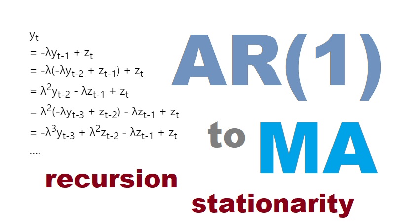
y_t 
= -λy_t-1 + z_t
= -λ(-λy_t-2 + z_t-1) + z_t
= λ²y_t-2 – λz_t-1 + z_t
= λ²(-λy_t-3 + z_t-2) – λz_t-1 + z_t
= -λ³y_t-3 + λ²z_t-2 – λz_t-1 + z_t
….

Since λ is the multiplier for R_t−1, it should be smaller than one as the effect of R_t−1 dies off over time.

Therefore, as we keep replacing y_t-k, the y-term eventually gets multiplied by a very small value of λ^k and becomes insignificant.

Therefore,

y_t = sum of (-λ)^kz_t-k for k from 0 to infinity 

Since 

y_t = (R_t – μ)/σ
R_t = σy_t + μ

Since y_t only depends on values of z_t-k, R_t only depends on z_t-k too, where k>=0.

In other words, R_t only depends on current and past values of z. We have successfully converted it to a MA model.

Useful conclusion:

E[z_sy_t] = 0 for t < s

This means z_s and y_t are independent. Put it another way, y_t does not depend on z_s, where s is a future time compared to t. Therefore,

E[z_t(R_t-1 – μ)] = 0

which is an intuitive property that we stated when solving the AR(1) model previously.