Import Libraries

In [1]:
# Import required libraries
import pandas as pd
import numpy as np

import warnings
warnings.filterwarnings('ignore')

# Get data
from sklearn.datasets import load_boston
from sklearn.metrics import mean_squared_error

Get Data

In [2]:
# Load data
boston_data = load_boston()
In [3]:
# Define feature and target
X = boston_data['data']        # Feature
y = boston_data['target']      # Label
In [4]:
# Subsume into a dataframe
boston = pd.DataFrame(boston_data['data'], columns=boston_data['feature_names'])
boston.head()
Out[4]:
CRIM ZN INDUS CHAS NOX RM AGE DIS RAD TAX PTRATIO B LSTAT
0 0.00632 18.0 2.31 0.0 0.538 6.575 65.2 4.0900 1.0 296.0 15.3 396.90 4.98
1 0.02731 0.0 7.07 0.0 0.469 6.421 78.9 4.9671 2.0 242.0 17.8 396.90 9.14
2 0.02729 0.0 7.07 0.0 0.469 7.185 61.1 4.9671 2.0 242.0 17.8 392.83 4.03
3 0.03237 0.0 2.18 0.0 0.458 6.998 45.8 6.0622 3.0 222.0 18.7 394.63 2.94
4 0.06905 0.0 2.18 0.0 0.458 7.147 54.2 6.0622 3.0 222.0 18.7 396.90 5.33

Explore Data

In [5]:
boston.shape
Out[5]:
(506, 13)
In [6]:
# Verify missing values on features
boston.isnull().sum()
Out[6]:
CRIM       0
ZN         0
INDUS      0
CHAS       0
NOX        0
RM         0
AGE        0
DIS        0
RAD        0
TAX        0
PTRATIO    0
B          0
LSTAT      0
dtype: int64
In [7]:
# Verify missing values on labels
pd.DataFrame(y).isnull().sum()
Out[7]:
0    0
dtype: int64
In [8]:
boston.describe()
Out[8]:
CRIM ZN INDUS CHAS NOX RM AGE DIS RAD TAX PTRATIO B LSTAT
count 506.000000 506.000000 506.000000 506.000000 506.000000 506.000000 506.000000 506.000000 506.000000 506.000000 506.000000 506.000000 506.000000
mean 3.613524 11.363636 11.136779 0.069170 0.554695 6.284634 68.574901 3.795043 9.549407 408.237154 18.455534 356.674032 12.653063
std 8.601545 23.322453 6.860353 0.253994 0.115878 0.702617 28.148861 2.105710 8.707259 168.537116 2.164946 91.294864 7.141062
min 0.006320 0.000000 0.460000 0.000000 0.385000 3.561000 2.900000 1.129600 1.000000 187.000000 12.600000 0.320000 1.730000
25% 0.082045 0.000000 5.190000 0.000000 0.449000 5.885500 45.025000 2.100175 4.000000 279.000000 17.400000 375.377500 6.950000
50% 0.256510 0.000000 9.690000 0.000000 0.538000 6.208500 77.500000 3.207450 5.000000 330.000000 19.050000 391.440000 11.360000
75% 3.677083 12.500000 18.100000 0.000000 0.624000 6.623500 94.075000 5.188425 24.000000 666.000000 20.200000 396.225000 16.955000
max 88.976200 100.000000 27.740000 1.000000 0.871000 8.780000 100.000000 12.126500 24.000000 711.000000 22.000000 396.900000 37.970000
In [9]:
print(boston_data['DESCR'])
.. _boston_dataset:

Boston house prices dataset
---------------------------

**Data Set Characteristics:**  

    :Number of Instances: 506 

    :Number of Attributes: 13 numeric/categorical predictive. Median Value (attribute 14) is usually the target.

    :Attribute Information (in order):
        - CRIM     per capita crime rate by town
        - ZN       proportion of residential land zoned for lots over 25,000 sq.ft.
        - INDUS    proportion of non-retail business acres per town
        - CHAS     Charles River dummy variable (= 1 if tract bounds river; 0 otherwise)
        - NOX      nitric oxides concentration (parts per 10 million)
        - RM       average number of rooms per dwelling
        - AGE      proportion of owner-occupied units built prior to 1940
        - DIS      weighted distances to five Boston employment centres
        - RAD      index of accessibility to radial highways
        - TAX      full-value property-tax rate per $10,000
        - PTRATIO  pupil-teacher ratio by town
        - B        1000(Bk - 0.63)^2 where Bk is the proportion of blacks by town
        - LSTAT    % lower status of the population
        - MEDV     Median value of owner-occupied homes in $1000's

    :Missing Attribute Values: None

    :Creator: Harrison, D. and Rubinfeld, D.L.

This is a copy of UCI ML housing dataset.
https://archive.ics.uci.edu/ml/machine-learning-databases/housing/


This dataset was taken from the StatLib library which is maintained at Carnegie Mellon University.

The Boston house-price data of Harrison, D. and Rubinfeld, D.L. 'Hedonic
prices and the demand for clean air', J. Environ. Economics & Management,
vol.5, 81-102, 1978.   Used in Belsley, Kuh & Welsch, 'Regression diagnostics
...', Wiley, 1980.   N.B. Various transformations are used in the table on
pages 244-261 of the latter.

The Boston house-price data has been used in many machine learning papers that address regression
problems.   
     
.. topic:: References

   - Belsley, Kuh & Welsch, 'Regression diagnostics: Identifying Influential Data and Sources of Collinearity', Wiley, 1980. 244-261.
   - Quinlan,R. (1993). Combining Instance-Based and Model-Based Learning. In Proceedings on the Tenth International Conference of Machine Learning, 236-243, University of Massachusetts, Amherst. Morgan Kaufmann.

Overview of Scikit-Learn's API

Data Preprocessing

In [10]:
from sklearn.preprocessing import StandardScaler

# create and fit scaler
scaler = StandardScaler()
scaler.fit(X)

# scale data set
Xt = scaler.transform(X)

Model Training

Using Linear Regression

In [11]:
from sklearn.linear_model import LinearRegression, Lasso, Ridge

# Train Linear Regression model
model = LinearRegression()
model.fit(X, y) # training

# Predict label values on X
y_pred = model.predict(X) # predicting

print(y_pred[:10])
print(f'R2 Score: {model.score(X, y):0.4}')
[30.00384338 25.02556238 30.56759672 28.60703649 27.94352423 25.25628446
 23.00180827 19.53598843 11.52363685 18.92026211]
R2 Score: 0.7406

How to improve R2 Score

  • Remove outliers
  • Test for multicollinearity and remove features
  • Change the predictor

Using Gradient Boosting (Ensemble method)

In [12]:
from sklearn.ensemble import GradientBoostingRegressor

# create model and train/fit
model = GradientBoostingRegressor()
model.fit(X, y)

# predict label values on X
y_pred = model.predict(X)

print(y_pred[:10])
print(f'R2 Score: {model.score(X, y):0.4}')
[25.90772604 21.96320179 33.92712155 34.14528061 35.41267912 26.7925396
 21.48031031 20.87839556 16.95411564 18.45898255]
R2 Score: 0.9761

Pipeline and FeatureUnion

Pipeline

  • Predictor is always the last step in a pipeline
  • Pipeline arranges estimators in a series

FeatureUnion

  • FeatureUnion arranges transformers in parallel
  • It combines the output of the each of the transformers in parallel to generate one output matrix

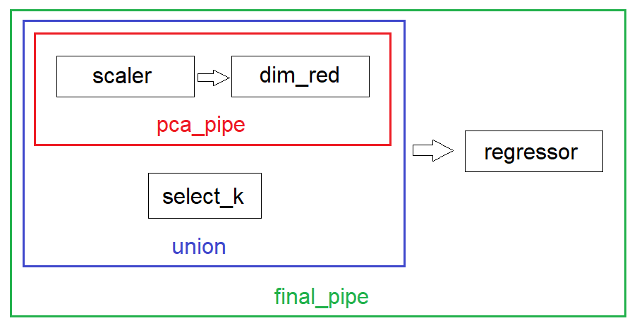
In the code below, pca_pipe gives us 4 features and selector gives us 2. Hence, we train our LinearRegression model using a total of 6 features.

In [13]:
from sklearn.pipeline import Pipeline, FeatureUnion
from sklearn.decomposition import PCA
from sklearn.feature_selection import f_regression, SelectKBest

# pca_pipe combines the scaling and dimensionality reduction steps
pca_pipe = Pipeline([('scaler', StandardScaler()), ('dim_red', PCA(n_components=4))])

# union combines pca_pipe with select_k in parallel to give us 6 features
union = FeatureUnion([('pca_pipe', pca_pipe), ('select_k', SelectKBest(f_regression, k=2))])

Training the model using a new pipeline final_pca

In [14]:
# final_pipe passes the 6 features to the predictor
final_pipe = Pipeline([('union', union), ('regressor', LinearRegression())]) # predictor is the last step
final_pipe.fit(X, y)
Out[14]:
Pipeline(memory=None,
         steps=[('union',
                 FeatureUnion(n_jobs=None,
                              transformer_list=[('pca_pipe',
                                                 Pipeline(memory=None,
                                                          steps=[('scaler',
                                                                  StandardScaler(copy=True,
                                                                                 with_mean=True,
                                                                                 with_std=True)),
                                                                 ('dim_red',
                                                                  PCA(copy=True,
                                                                      iterated_power='auto',
                                                                      n_components=4,
                                                                      random_state=None,
                                                                      svd_solver='auto',
                                                                      tol=0.0,
                                                                      whiten=False))],
                                                          verbose=False)),
                                                ('select_k',
                                                 SelectKBest(k=2,
                                                             score_func=<function f_regression at 0x0000013D840D9C10>))],
                              transformer_weights=None, verbose=False)),
                ('regressor',
                 LinearRegression(copy_X=True, fit_intercept=True, n_jobs=None,
                                  normalize=False))],
         verbose=False)

Overview of the Pipeline and FeatureUnion objects

Printing outputs of pca_pipe and union

In [15]:
pca_pipe.fit_transform(X)
Out[15]:
array([[-2.09829747,  0.77311275,  0.34294273, -0.89177403],
       [-1.45725167,  0.59198521, -0.69519931, -0.48745853],
       [-2.07459756,  0.5996394 ,  0.1671216 , -0.73920419],
       ...,
       [-0.31236047,  1.15524644, -0.40859759, -0.78630409],
       [-0.27051907,  1.04136158, -0.58545406, -0.67813391],
       [-0.12580322,  0.76197805, -1.294882  , -0.2883292 ]])

As shown above, we end up with 4 features. For instance, for the first instance in the dataset, we end up with 4 features (i.e. dimensions) of values -2.09829747, 0.77311275, 0.34294273 and -0.89177403.

In [16]:
union.fit_transform(X, y)
Out[16]:
array([[-2.09829747,  0.77311275,  0.34294273, -0.89177403,  6.575     ,
         4.98      ],
       [-1.45725167,  0.59198521, -0.69519931, -0.48745853,  6.421     ,
         9.14      ],
       [-2.07459756,  0.5996394 ,  0.1671216 , -0.73920419,  7.185     ,
         4.03      ],
       ...,
       [-0.31236047,  1.15524644, -0.40859759, -0.78630409,  6.976     ,
         5.64      ],
       [-0.27051907,  1.04136158, -0.58545406, -0.67813391,  6.794     ,
         6.48      ],
       [-0.12580322,  0.76197805, -1.294882  , -0.2883292 ,  6.03      ,
         7.88      ]])

Here, we end up with six features. The first 4 are from pca_pipe while the additional two are from select_k.

Custom Transformer

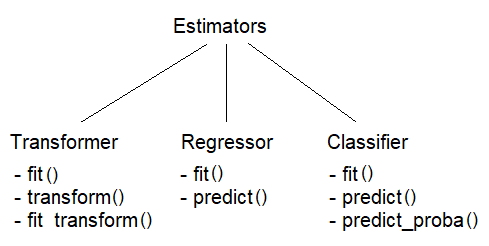
Scikit-learn has a base class called BaseEstimator that all estimators inherit.

Depending on the estimator type, they also inherit mixin classes such as RegressorMixin (for regressors), ClassifierMixin (for classifiers), and TransformerMixin (for transformers).

We can customize models by inheriting these classes and leverage on sklearn's functionalities such as Pipeline, GridSearchCV and such other features.

Description

In the code sample below, we create three variables X1, X2, and y, where y = X1 + 2*np.sqrt(X2).

If we try to use a linear regression model to fit these data, the model will not fit perfectly.

However, if we transform X2 to X2 = 2*np.sqrt(X2), we now have a perfect linear relationship, where y = X1 + X2. Training a linear regression model using X1, X2, and y will now give us a perfect fit (where RMSE = 0).

The code below demonstrates how to create a custom transformer to transform X2 to X2 = 2*np.sqrt(X2).

Code

In [17]:
# Creating X1, X2, and y and adding them to a DataFrame df

X1 = np.arange(1,21)
X2 = np.arange(11,31)
y = X1 + 2*np.sqrt(X2)

df = pd.DataFrame({'X1':X1, 'X2':X2, 'y': y}, columns = ['X1', 'X2', 'y'])
print(df.head())
   X1  X2          y
0   1  11   7.633250
1   2  12   8.928203
2   3  13  10.211103
3   4  14  11.483315
4   5  15  12.745967
In [18]:
# Split into training and test subsets (80:20)

train_X = df.iloc[:16, :-1]
test_X = df.iloc[16:, :-1]

train_y = df.iloc[:16, -1]
test_y = df.iloc[16:, -1]
In [19]:
# Training the model

lr1 = LinearRegression()
lr1.fit(train_X, train_y)
pred_y1 = lr1.predict(test_X)

print(f'{pred_y1}')
print(f'RMSE: {np.sqrt(mean_squared_error(test_y, pred_y1))}')
[27.5384685 28.7743983 30.0103281 31.2462579]
RMSE: 0.2240231957964702
In [20]:
# Creating a custom transformer to transform X2 and train the linear regression model

from sklearn.base import BaseEstimator, TransformerMixin

# Build custom transformer SQRTTransformer that inherits BaseEstimator and TransformerMixin
class SQRTTransformer(BaseEstimator, TransformerMixin):
    def __init__(self, feature):
        self.feature = feature
    
    def fit(self, X, y=None):
        return self
    
    def transform(self, X):
        Xt = X.copy()
        Xt[self.feature] = 2 * np.sqrt(Xt[self.feature])
        return Xt
In [21]:
# Training the model again

pipe = Pipeline([('sqrt_trans', SQRTTransformer('X2')), # user defined
                 ('regressor', LinearRegression())]) # from sklearn

pipe.fit(train_X, train_y)
pred_y2 = pipe.predict(test_X)

print(f'{pred_y2}')
print(f'RMSE: {np.sqrt(mean_squared_error(test_y, pred_y2)):.0f}')
[27.39230485 28.58300524 29.77032961 30.95445115]
RMSE: 0

Custom Regressor

In the code sample below, we build a custom regression that returns the mean of the y values passed to its fit() method.

In [22]:
from sklearn.base import RegressorMixin

# Build regressor
class MeanRegressor(BaseEstimator, RegressorMixin):
    def __int__(self):
        pass
    
    def fit(self, X, y):
        self.y_mean = np.mean(y)
        return self
    
    def predict(self, X):
        return self.y_mean * np.ones(X.shape[0])
In [23]:
# Training a MeanRegressor model

mr = MeanRegressor()

mr.fit(train_X, train_y)
results = mr.predict(test_X)

results
Out[23]:
array([17.0330652, 17.0330652, 17.0330652, 17.0330652])

Let's verify that 17.0330652 is indeed the mean of train_y

In [24]:
train_y.mean()
Out[24]:
17.033065200308354
In [25]:
# Evaluating the performance of mr

print(f"R2 score: {mr.score(train_X, train_y)}")   # score method inherited from base class
R2 score: 0.0

As expected, mr offers no improvement over using the mean as the predictor since all that it does is return the mean of the y values.