In this post, we are going to scale the random walk to change it from a discrete time model to a continuous time model. This is going to give us a Brownian motion.
Let us first declare Ba,b as a Brownian motion with a time step of “a” and a total duration of “b”.
We can rewrite our basic random walk model as a Brownian motion with a discrete time step of 1 and a total time of T. This gives us
\begin{aligned}
\text{Random Walk} &= B_{1, T}\\
&= \sum\limits_{t=t_0 + 1}^{t_0 + T} z_t, \text{where }t_0\text{ is the initial time}
\end{aligned}Testing Three Models
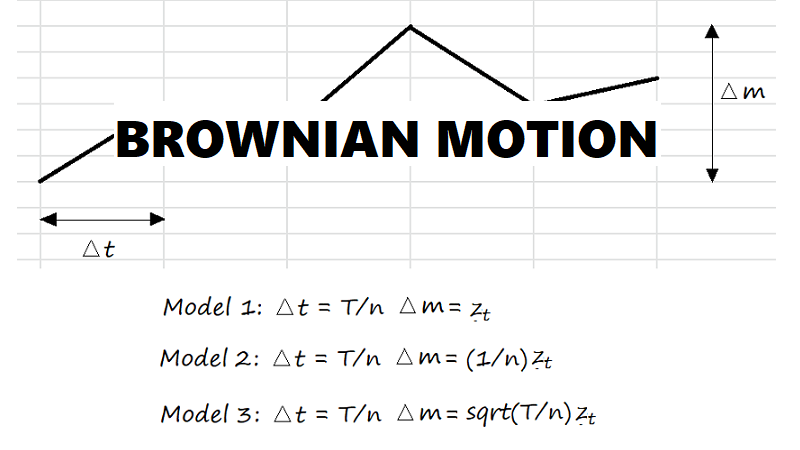
To scale this random walk into a continuous model, we’ll consider three different scalings.
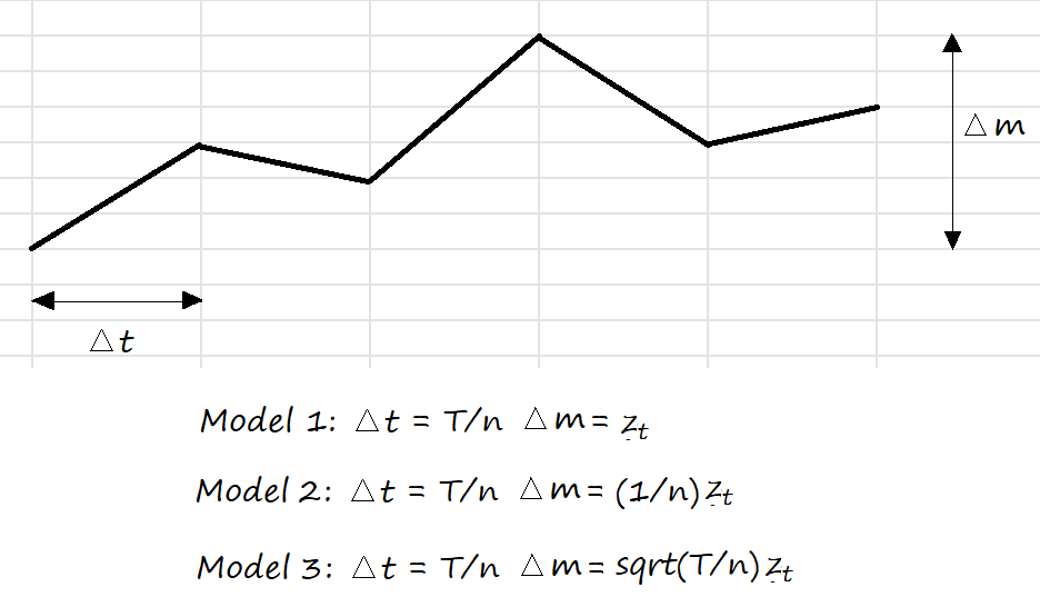
MODEL 1: Smaller Time Steps
First, let’s consider smaller time steps. Instead of a time step of 1, let’s use a time step of T/n.
\begin{aligned}
Let\ \Delta t &= \frac{T}{n}\\\\
B_{\Delta t, T} &= \sum\limits_{t=1}^{n} z_t\\\\
E[B_{\Delta t, T}] &= 0\\\\
Var(B_{\Delta t, T})
&= nVar(z_t) \\
&= n
\end{aligned}Var(BΔt, T) tends to infinity as n tends to infinity. Hence, this model does not work as it does not converge.
MODEL 2: Smaller Time and Movement Step (Movement Step = 1/n)
\begin{aligned}
\text{Let }\Delta t = \frac{T}{n}, \;\epsilon_t &= \lambda z_t, \;\lambda =\frac{1}{n}\\\\
B_{\Delta t, T} &= \sum\limits_{t=1}^{n} \epsilon_t\\
&= \lambda\sum\limits_{t=1}^{n} z_t\\\\
E[B_{\Delta t, T}] &= 0\\\\
Var(B_{\Delta t, T})
&= nVar(\epsilon_t) \\
&= nVar(\lambda z_t) \\
&= n\lambda^2Var(z_t)\\
&= n\lambda^2\\
&= \frac{n}{n^2}\\
&= \frac{1}{n}
\end{aligned}Var(BΔt, T) tends to zero as n tends to infinity. Hence, this model is not useful as there is no randomness at all.
MODEL 3: Smaller Time and Movement Steps (Movement Step = sqrt(T/n))
\begin{aligned}
\text{Let }\Delta t = \frac{T}{n}, \;\epsilon_t &= \lambda z_t, \;\lambda = \sqrt{\frac{T}{n}}\\\\
B_{\Delta t, T} &= \sum\limits_{t=1}^{n} \epsilon_t\\
&= \lambda\sum\limits_{t=1}^{n} z_t\\\\
E[B_{\Delta t, T}] &= 0\\\\
Var(B_{\Delta t, T})
&= nVar(\epsilon_t) \\
&= nVar(\lambda z_t) \\
&= n\lambda^2Var(z_t)\\
&= n\lambda^2\\
&= n\left(\frac{T}{n}\right) \\
&= T
\end{aligned}Var(BΔt, T) is finite and non-zero.
Therefore, lim BΔt, T as Δt tends to zero ~ N(0, T)
Properties of Brownian Motion
Property 1
Let X be a Brownian motion that goes between t1 and t2.
X(t_1, t_2) = B(t_2) - B(t_1)\\\\
X \sim N(0, t_2 - t_1), \quad t < t_1 \leqslant t_2
Properties and distribution of X only depend on t2 – t1.
Property 2
Previously, we let Δt = T/n, where T is a finite time duration.
Now, let T become smaller and smaller until T = dt. We’ll denote the path in that time interval as dBt.
A brownian path is Guassian at all time scales. Therefore,
dB_t \sim N(0, dt)\\
\begin{aligned}
\\Cov(dB_t, dB_{t'}) &= dt \text{ if t = t', 0 otherwise}\\
\int_{0}^T dB_t &= B(T) - B(0)
\end{aligned}
Scaling for Drift and Volatility
For Δt = 1 (i.e. a discrete time step of 1 unit)
\begin{aligned}
r_t &= log(\frac{S_t}{S_{t-1}})\\
&= \mu_0 + \sigma_0z_t\\
\end{aligned}
\\
r_t\sim N(\mu_0, \sigma_0^2)\\

\begin{aligned}
\\log(\frac{S_T}{S_0}) &= log\left(\frac{S_T}{S_{T-1}}\frac{S_{T-1}}{S_{T-2}}...\frac{S_{1}}{S_{0}}\right)\\
&= r_T + r_{T-1} + ... + r_1\\
&\sim N(T\mu_0, T\sigma_0^2)
\end{aligned}
Let Δt = T/n, εt = λzt, λ = (T/n)0.5
\begin{aligned}
\\log(\frac{S_T}{S_0})
&= \lim_{\Delta t \to 0} \left[\sum_{t=1}^{n}(\mu\Delta t) + \sum_{t=1}^{n}(\sigma z_t \sqrt{\Delta t})    \right]\\
&= \lim_{\Delta t \to 0} \left[n(\mu\Delta t) + \sigma\sum_{t=1}^{n}(z_t \sqrt{\Delta t})    \right]\\
&= \lim_{\Delta t \to 0} \left[\mu T + \sigma\sum_{t=1}^{n}\epsilon_t    \right]\\
&= \mu T + \sigma \int dB_t \\
&\sim N(T\mu, T\sigma^2)
\end{aligned}
If drift and volatility are not constants and depend on time deterministically,
log\left( \frac{S_{t_2}}{S_{t_1}}\right) = \int_{t_1}^{t_2} \sigma(t)dB_t
Leave a Reply