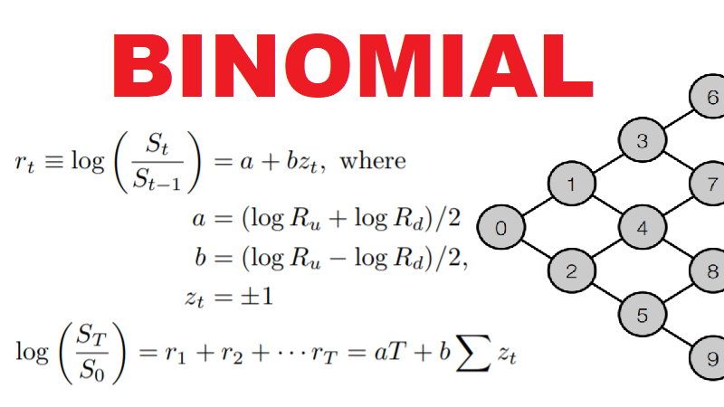
A binomial model is made up of nodes that split into two separate branches.
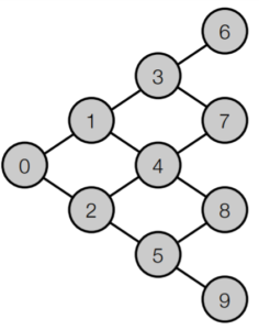
Suppose the branches in the model above represent log returns rt and the nodes represent asset values St.
We can represent the model using the equations below:
\begin{aligned}
r_t &\equiv log\left(\frac{S_t}{S_{t-1}}\right) \\
&= a + bz_t, \text{ where }z_t = \pm 1\text{ and}\\
\\
a &= \frac{logR_u + logR_d}{2}\\
b &= \frac{logR_u - logR_d}{2}. \\
\\
\text{Therefore, }\frac{S_t}{S_{t-1}} &= R_u \text{ when z = 1 (i.e. an up move) and }\\
&= R_d \text{ when z = -1 (i.e. a down move)}\\
\\
log\left(\frac{S_T}{S_0}\right) &= log\left(\frac{S_T}{S_{T-1}}\right) + log\left(\frac{S_{T-1}}{S_{T-2}}\right) + ... + log\left(\frac{S_1}{S_0}\right)\\
&= r_T + ... + r_2 + r_1\\
&= aT + b\sum z_t\\

\end{aligned}
If we let X = log(ST/S0), we can rewrite the equation above as
\begin{aligned}
X &= r_1 + r_2 + ...+ r_T\\
\end{aligned}
This is essentially a generalized random walk model, where
\begin{aligned}
r_t &= a + bz_t,\;z_t = \pm1\\
\end{aligned}
In other words, we can create a random walk model using a binomial model.
Let’s look at a concrete example:
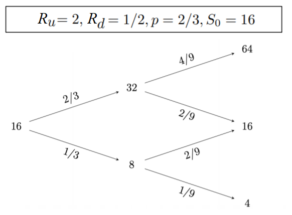
Consider the case where S2 = 64
\begin{aligned}
X &= log\left(\frac{64}{16}\right)\\
&= r_1 + r_2\\
&= log\left(\frac{32}{16}\right) + log\left(\frac{64}{32}\right)\\
&= a + b(1) + a + b(1)\\
&= 2a + 2b\\
&= log(2) + log(2)\\
&= log(4)
\end{aligned}
To connect the model to real-world asset prices, we can calculate the mean and variance of the model.
\begin{aligned}
\mu &= E[r_t]\\
&= E[a + bz_t]\\
&= a + pb\text{ (where p = P(}z_t = 1))\\
\\
\sigma^2 &= Var(r_t)\\
&= E[(r_t - a - pb)^2]\\
&= E[(bz_t - pb)^2]\\
&= b^2E[(z_t - p)^2]\\
&= b^2\{E[z_t^2] - 2E[z_tp] + E[p^2]\}\\
&= b^2\{E[z_t^2] - 2E[z_tp] + E[p^2]\}\\
&= b^2(p - 2p^2 + p^2)\\
&= b^2p(1-p)
\end{aligned}
Leave a Reply